
Fault analysis of mixing quality using Laplace transform
The Laplace transform is a mathematical calculation method for control systems to switch from the "time domain" to the "frequency domain."
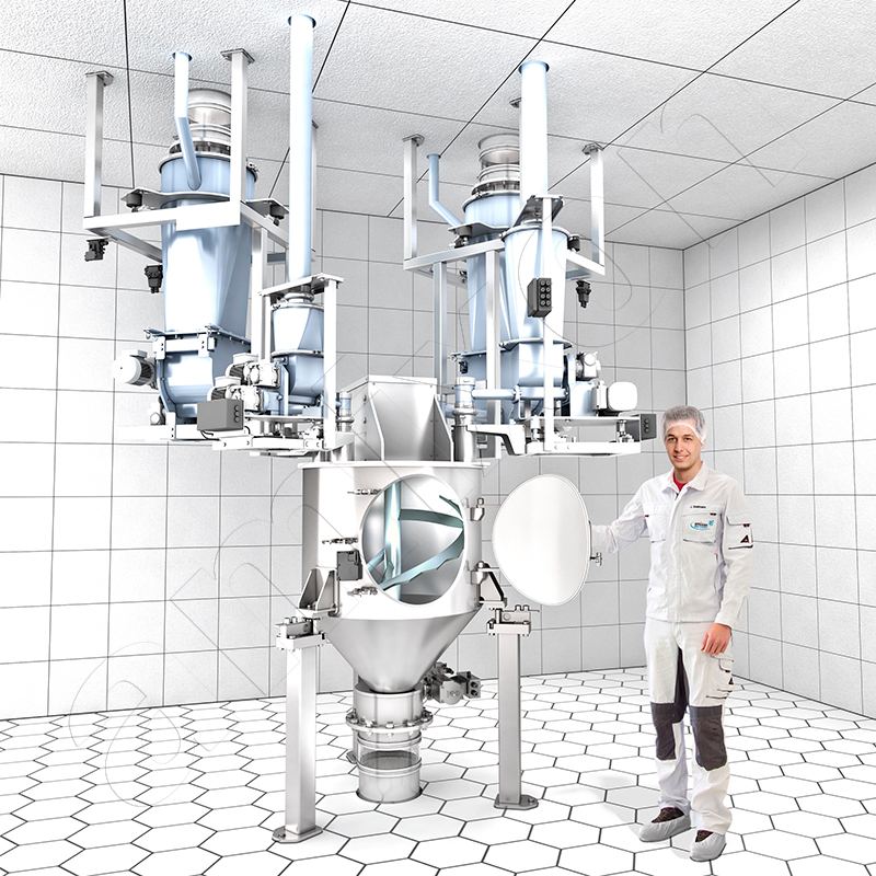
Example application of the Laplace transformation for a continuous mixing process in the amixon® AMK 1000 mixer: Powder A flows constantly into the mixer at a rate of 1,000 kg/h. Powder B is dosed simultaneously at a rate of 10 kg/h. The mixing chamber remains closed at the start. The mixing tool is already running and achieves ideal mixing quality after 20 revolutions. It rotates at 20 rpm.
As soon as 700 kg of product are present in the mixer, the discharge valve opens. The discharge is adjusted so that the incoming 1,010 kg/h are also discharged again. The process runs smoothly.
Suddenly, a malfunction occurs: the supply of component B stops completely for 20 seconds. Afterwards, the dosing device is corrected and B flows at double the rate (20 kg/h) for 20 seconds. The flow then stabilises again at 10 kg/h.
Before the malfunction, the mixing quality was technically ideal. The coefficient of variation for the mixing quality was 3%.
Process in figures (initial situation)
Inlet A: ṁ_A = 1000 kg/h; Inlet B (nominal): ṁ_B = 10 kg/h; Total inlet: ṁ_in = 1010 kg/h. Constant powder mass in the mixer: M = 700 kg.
Average residence time τ (time constant):
t = M / ṁ_aus = 700 / 1010 h = 0.693 h = 41.6 min = 2495 s
Nominal mass fraction of B at the inlet (and stationary at the outlet):
x_B,in,0 = 10 / 1010 = 0.00990099 (≈ 0.9901 %)
Interference scenario (inflow B)
0 ≤ t < 20 s: Blockade, ṁ_B = 0; 20 ≤ t < 40 s:
Correction, ṁ_B = 20 kg/h; t ≥ 40 s: again 10 kg/h.
We consider the deviation of the B fraction in the inflow relative to the nominal fraction:
u(t) = x_B,in(t) − x_B,in,0.
Piecewise definition (total flow approximately constant at 1010 kg/h):
u(t) = {-x_B,in,0 for 0≤t<20 s; +x_B,in,0 for 20≤t<40 s; 0 for t≥40 s}
Dynamic model (PT1, ideally mixed)
Outlet fraction y(t) (deviation of the B fraction at the outlet) follows a PT1 model:
dy(t)/dt + y(t) = u(t), y(0⁻) = 0
Outlet fraction y(t) (deviation of the B fraction at the outlet) follows a PT1 model:
dy(t)/dt + y(t) = u(t), y(0⁻) = 0
Laplace solution
Laplace transform of PT1:
Y(s) = (1 / (τ s + 1)) · U(s)
τ (tau): the time constant of the system (here: the average residence time in the mixer)
s: the Laplace variable, a measure of how signals change over time
"τ · s" is a dimensionless combination of time constant and rate of change.
Input u(t) as the difference between two rectangular jumps; with Heaviside shifts, this results in:
U(s) = x_B,in,0 · (-1 + 2 e^{-20 s} - e^{-40 s}) / s
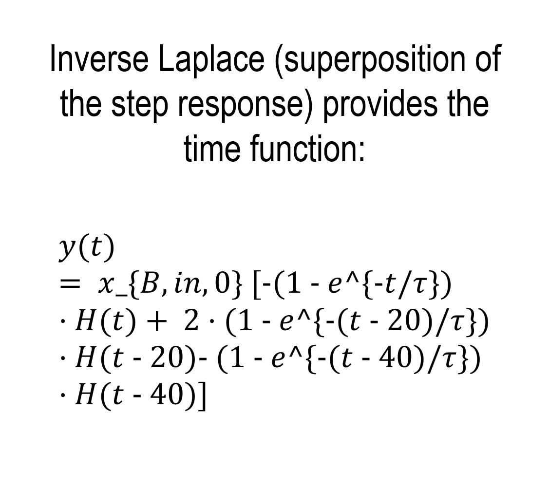
Time domain solution (superposition of step responses, Heaviside H(·)):
y(t)=x_B,in,0[ - (1 - e^{-t/τ}) H(t) + 2 (1 - e^{-(t-20)/τ}) H(t-20) - (1 - e^{-(t-40)/τ}) H(t-40) ]
Laplace transform of PT1:
Y(s) = (1 / (τ s + 1)) · U(s)
τ (tau): the time constant of the system (here: the average residence time in the mixer)
s: the Laplace variable, a measure of how signals change over time
"τ · s" is a dimensionless combination of time constant and rate of change.
Input u(t) as the difference between two rectangular jumps; with Heaviside shifts, this results in:
U(s) = x_B,in,0 · (-1 + 2 e^{-20 s} - e^{-40 s}) / s
Time domain solution (superposition of step responses, Heaviside H(·)):
y(t)=x_B,in,0[ - (1 - e^{-t/τ}) H(t) + 2 (1 - e^{-(t-20)/τ}) H(t-20) - (1 - e^{-(t-40)/τ}) H(t-40) ]
Numerical values and maximum deviation
With τ = 2495 s and x_B,in,0 = 0.00990099, the results are:
e^{-20/τ} = e^{-20/2495} ≈ 0.99202; 1 - e^{-20/τ} ≈ 0.00798
Largest negative deviation at the end of the blockage (t = 20 s):
y(20) = - x_B,in,0 (1 - e^{-20/τ}) ≈ -7.9·10^{-5} (≈ -0.0079 % absolute)
End of overdose (t = 40 s):
y(40) ≈ +6.3·10^{-7} (practically nominal)
For t > 40 s, the tiny residual deviation decays exponentially:
y(t) = y(40) · e⁻^(t-40)/τ
Classification according to mix quality (CV = 3%)
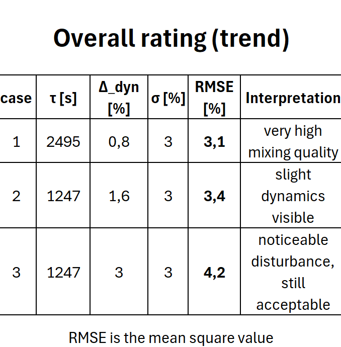
The dynamic deviation of the B fraction (~0.8% relative) caused by the disturbance is significantly below the specified coefficient of variation for the mix quality (3%). The disturbance is therefore practically invisible in the product stream.
The dynamic deviation of the B fraction (~0.8% relative) caused by the disturbance is significantly below the specified coefficient of variation for the mix quality (3%). The disturbance is therefore practically invisible in the product stream.
Benefits of Laplace analysis
The Laplace representation provides a closed formula for the temporal effect of inflow profiles on the outlet mixing quality. This allows maximum deviations, recovery times and the influence of the residence time to be quickly estimated – helpful for the design of mixing chambers and correction strategies.
The Laplace representation provides a closed formula for the temporal effect of inflow profiles on the outlet mixing quality. This allows maximum deviations, recovery times and the influence of the residence time to be quickly estimated – helpful for the design of mixing chambers and correction strategies.
How does the mixing quality change when the mass flows are twice as large?
How does the mixing quality change when the mass flows are doubled and the average residence time is reduced from 41.6 minutes to 20.8 minutes? Powder A now flows at 2,000 kg/h instead of 1,000 kg/h. Powder B now flows at 20 kg/h instead of 10 kg/h. This is the same AMK 1000 continuous mixer with a rotation frequency of 20 rpm, a filling level of 700 kg and the same components A and B. The fault is the same: component A flows continuously, component B is blocked for 20 seconds, then component B flows at double the rate for 20 seconds. The components then flow as normal.
Conclusion
The relative deviation at the outlet is now approximately 1.6% (previously 0.8%). Since the dwell time has been halved, the system reacts twice as fast and shows an amplitude deviation that is approximately twice as large. The nominal fraction remains unchanged, so the effect scales directly with 1 - e^{-20/τ}.
Classification of mixing quality (CV = 3 %)
The 1.6 % relative dynamic deviation is also below the coefficient of variation of the mixing quality (3 %). The disturbance remains moderate in the product stream, but is visibly stronger than in the first case.
What happens if the dynamic deviation is 3%?
What happens if the dynamic deviation is 3% (instead of 1.6%) and is therefore in the order of magnitude of the ‘basic dispersion’ (CV = 3%)? How should the change in mixing quality be assessed if, due to a major disturbance, the relative dynamic deviation is now 3% instead of 1.6%? Similar to disturbance-free operation?
- The dynamic deviation is now in the order of magnitude of the stationary CV.
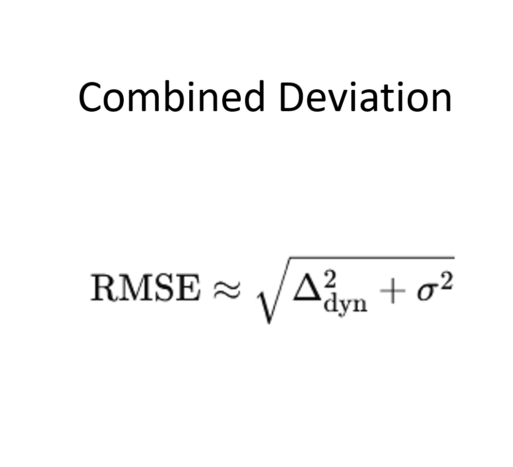
- The total deviation increases to over 4%.
- Quality usually remains within ±5%, but the risk of outliers increases significantly.
The continuous mixer acts like a low-pass filter. Halving the residence time leads to approximately a doubling of the dynamic disturbance deviation. As long as this remains below the coefficient of variation, the process remains robust. If it becomes equal to or greater than this, it adds quadratically to the dispersion – the mixing quality deteriorates noticeably, but remains controllable for the time being.
What happens if the dynamic deviation is 3% (instead of 1.6%) and is therefore in the order of magnitude of the ‘basic dispersion’ (CV = 3%)? How should the change in mixing quality be assessed if, due to a major disturbance, the relative dynamic deviation is now 3% instead of 1.6%? Similar to disturbance-free operation?
- The dynamic deviation is now in the order of magnitude of the stationary CV.
- The total deviation increases to over 4%.
- Quality usually remains within ±5%, but the risk of outliers increases significantly.
The continuous mixer acts like a low-pass filter. Halving the residence time leads to approximately a doubling of the dynamic disturbance deviation. As long as this remains below the coefficient of variation, the process remains robust. If it becomes equal to or greater than this, it adds quadratically to the dispersion – the mixing quality deteriorates noticeably, but remains controllable for the time being.
© Copyright by amixon GmbH