Unbalance correction for rotating shafts

Case study: A horizontally rotating shaft is corrected a) statically and b) dynamically by specifically adding or removing mass in defined planes so that the resulting unbalance force or unbalance moment disappears or falls below a tolerance. Static balancing corrects a pure shift in the centre of gravity in one plane, while dynamic balancing additionally corrects tilting imbalance components by balancing in two (or more) planes along the shaft.

1. Imbalance and excitation frequency

A rotating shaft with imbalance is described by an eccentric mass. This imbalance mass has a magnitude of m_u and a distance of e from the axis of rotation. The imbalance product is U=m_u e. The shaft rotates at a speed of n revolutions per minute. This results in an excitation frequency in hertz of f=n/60. The corresponding angular velocity is Ω=2πf=2πn/60.

The unbalanced mass moves in a circular path and experiences a radial centrifugal force. The magnitude of this force is F_u=m_u eΩ^2=UΩ^2. For vibration excitation, the projection of this force in a fixed direction, for example vertically, is of interest. This projection changes harmonically with time. Therefore, the time-dependent excitation force is written as

F(t)=F₀ sin(Ωt)

The amplitude F₀ is equal to m_u e〖 Ω〗^2.

2. Static balancing

Static balancing involves examining a shaft that is essentially short and solid. The imbalance can then be modelled as a purely static imbalance. The shaft is mounted so that it rotates very smoothly and allowed to swing. The heaviest point comes to rest at the bottom and marks the direction of the centre of gravity. The aim is to correct the imbalance so that the centre of gravity is once again on the axis of rotation.

If a corrective weight m_K is attached within a radius r_K, its imbalance product must compensate for the original imbalance. The following applies

m_K r_K=m_u 

In practice, you can either remove material from the heavy area or attach a weight opposite it. Once the correction has been successfully completed, the shaft will remain in any angular position and will no longer wobble.

3. Dynamic balancing

Dynamic balancing also takes into account moment imbalance. Two correction planes are used along the shaft for this purpose. A correction weight with a specific mass and angular position can be attached to each plane. The shaft runs at low speed on a balancing machine or in its installed state. Vibrations and phase positions are measured at the bearings.

The measured vibration vectors are varied with test weights in both planes. The changes result in a linear system of equations that describes the influence of the correction masses. This system provides the optimum correction masses m_K1 and m_K2 as well as their angular positions. After attaching the correction weights, both force imbalance and moment imbalance are greatly reduced, and the shaft runs more smoothly at operating speed.

4. Spring stiffness of the beam

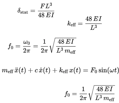
For vibration calculations, the shaft is often described by a substitute system with a mass and a spring. The vertical stiffness of a simply supported beam with span L and bending stiffness EI is determined by the static deflection. A single load F is considered in the centre of the beam. The deflection in the centre is

δ=(FL^3)/48EI

The effective spring stiffness in the centre is calculated as k=F/δ. This gives

k=48EI/L^3 

5. Effective mass and natural frequency

The oscillating mass consists of the machine mass and a portion of the beam mass. An effective mass m_eff is defined. This is approximately m_eff=m_M+ηm_B. Here, m_M is the mass of the machine and m_B is the mass of the support. The participation factor η is typically in the range of about 0.2 to 0.3. If the machine is much heavier than the support, m_eff≈m_M is used as an approximation.

The system consisting of spring stiffness k and mass m_eff forms a single-mass oscillator. The equation of motion without damping is

m_eff  x ¨(t)+kx(t)=0

The natural frequency follows from this equation

ω_0=√(k/m_eff )

The natural frequency in hertz is

f_0=ω_0/2π

If k=48EI/L^3 is used for the beam, the result is

f_0=1/2π √(48EI/(L^3 m_eff ))

This relationship shows that the natural frequency increases with bending stiffness and decreases with increasing span and mass.

6. Resonance analysis

To assess the risk of resonance, the excitation frequency of the imbalance is compared with the natural frequency. The excitation frequency is f=n/60. The natural frequency is f_0. If both values are close to each other, resonance is likely to occur. If f is significantly below or significantly above f_0, the risk of resonance is lower. In practice, a safety margin is provided so that the resonance range does not occur during continuous operation.