Mixing efficiency

Mixing efficiency describes the ratio of the effectiveness of a mixing process to the time or energy required for it. It indicates how effectively a mixer or mixing process reduces existing concentration differences in the product and achieves a specified homogeneity. Since mixed goods and process conditions vary, there is no universal formula for determining mixing efficiency. However, several methodological approaches have become established in industrial practice.

1. Variance or standard deviation-based mixing efficiency

Mixing efficiency is most commonly described in terms of the reduction in concentration variance. To do this, the variance of the mixing quality before the start of the mixing process is compared with the variance after a defined mixing time. The greater the reduction in variance, the more efficient the process.

The following formula is often used:

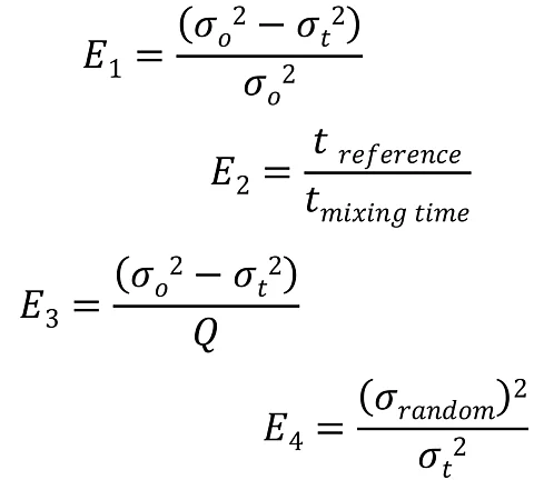
E₁ = (σ₀² − σₜ²) / σ₀²

σ₀² = initial variance of the mixture
σₜ² = variance after a specific mixing time t

Interpretation: E = 0 → no improvement, E = 1 → theoretically perfect homogeneity (σₜ² → 0). This ‘efficiency’ therefore describes the proportion of the original degree of inhomogeneity that has already been reduced.

2. Mixing efficiency in relation to mixing time

Another approach is based on the required mixing time. Here, efficiency is understood as the ability to achieve the desired homogeneity in the shortest possible time. Shorter mixing times correspond to higher mixing efficiency and allow conclusions to be drawn about the performance of the mixing tool and the flow mechanisms in the mixing chamber.

E₂ = t_reference / t_{mixing time}

Interpretation: The shorter the mixing time, the higher the efficiency.

3. Energetic mixing efficiency

In energy-intensive processes, especially in mixing processes with high shear or dispersion effects, mixing efficiency is often defined as the gain in homogeneity per unit of energy used. This approach takes into account the fact that, in addition to time, energy consumption is also a decisive factor in process evaluation.

E₃ = (σ₀² − σ_t²) / Q

Q = Energy consumption of the mixer. Interpretation: E is thus a measure of how ‘well’ a mixer produces homogeneity from the energy input.

4. Theoretical reference: Random mixing

In some applications, the variance actually achieved is also compared with the theoretical variance of an ideal random mixing process. This methodological comparison provides information on how close a mixing process comes to the statistically best possible result.

σ_random² = p · (1 − p) / n

σ²_random = variance of the theoretically ideal mixing quality
σ²_t = variance of the achieved mixing quality
p = material proportion of the component
n = number of particles in the sample volume

This results in:

E₄ = σ_random² / σ_t²

E > 1 means that the real process mixes ‘better than random’ (rare in practice).